Chapter 11 Quarks

In this section we will study the electromagnetic and weak interactions involving the 3 generations of quarks.

11.1 Electromagnetic interactions

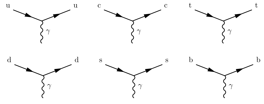
Since quarks are charged, they have electromagnetic interactions, which are summarised in Fig. 11.1.

Figure 11.1: The basic vertex summarising electromagnetic interactions involving quarks.

11.2 Quark conservation laws

Just as there are conservation laws for lepton quantum numbers, there are conservation laws for quark flavours. We start by considering strangeness, charm, truth, and beauty. Strangeness is defined by

$$S=-N_S=-[N(s)-N(\overline{s})],$$ (11.1)

where $N(s)$ is the number of strange quarks and $N(\overline{s})$ is the number of anti-strange quarks. Make note of the minus sign. The strangeness quantum number is the analogue of the lepton quantum number. Charm is defined as

$$C=N_C=[N(c)-N(\overline{c})],$$ (11.2)

Beauty is defined as

$$\tilde{B}=-N_B=-[N(b)-N(\overline{b})],$$ (11.3)

where $N(b)$ is the number of bottom quarks and $N(\overline{b}$) is the number of anti-bottom quarks. The little line, the tilde, is drawn across the letter $\tilde{B}$ so as to distinguish beauty from baryon number $B$. Truth is defined as

$$T=N_T=[N(t)-N(\overline{t})].$$ (11.4)

Here $N(t)$ is the number of top quarks, $N(\overline{t}$), the number of anti-top quarks. The up-ness and down-ness of quarks has been omitted from this scheme because they are included in the baryon number, $B$, and the charge baryon number, $Q$. The baryon number is defined as

$$B=\frac{1}{3}[N(q)-N(\overline{q})]$$ (11.5)

where $N(q)$ is the number of quarks, and $N(\overline{q})$ is the number of anti-quarks. Thus a meson has a quark and an anti-quark, so $B=0$. A meson has a baryon number of zero which makes sense since a meson is not a baryon. But since three quarks make a baryon we have $B=1$. An anti-baryon (e.g. an anti-proton) has a baryon number of $-1$. We can rewrite $B$ in terms of the quark numbers as

$B={\displaystyle \frac{1}{3}}[N_U+N_D+N_S+N_C+N_B+N_T]$

$={\displaystyle \frac{1}{3}}[N_U+N_D-S+C-\tilde{B}+T].$ (11.6)

Here $N_U$ is the number of up quarks and $N_D$ is the number of down quarks. The charge of baryons is

$Q={\displaystyle \frac{2}{3}}(N_U+N_C+N_T)-{\displaystyle \frac{1}{3}}(N_D+N_S+N_B)$ (11.7)

$={\displaystyle \frac{2}{3}}(N_U+C+T)-{\displaystyle \frac{1}{3}}(N_D-S-\tilde{B}).$

We could use $N_U$ and $N_D$ as quantum numbers, but instead use $B$ and $Q$ for the following reason. In the strong and electromagnetic interactions all the quark quantum numbers from Eqn. (11.1) to (11.7) are conserved (including $N_U$ and $N_D$). However, in the weak interaction, the individual quark flavour numbers can change, and only $B$ and $Q$ are conserved.

11.3 Charged current interactions

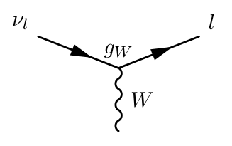
Charged current interactions are weak interactions involving $W^{\pm }$ bosons. Recall the basic vertex for $W^{\pm }$-lepton interactions, as shown in Fig. 11.2 (remember the charge on the $W$ is unspecified, depending on whether it is incoming or outgoing, and the corresponding anti-particle interactions are also implicit). The interaction occurs with a coupling strength $g_W$, where

$${\alpha }_W=\frac{g_W^2}{4\pi \mathrm{\hslash }c}.$$ (11.8)

Figure 11.2: The basic vertex for $W^{\pm }$-lepton interactions.

The concept of lepton universality states that $g_W$ is the same for each of the three generations

$$\left(\begin{array}{c}{\nu }_e\\ e^{-}\end{array}\right),\left(\begin{array}{c}{\nu }_{\mu }\\ {\mu }^{-}\end{array}\right),\left(\begin{array}{c}{\nu }_{\tau }\\ {\tau }^{-}\end{array}\right).$$

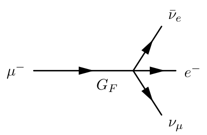
This can easily be tested experimentally. For example, consider the decays ${\mu }^{-}\to e^{-}+{\overline{\nu }}_e+{\nu }_{\mu }$ and ${\tau }^{-}\to e^{-}+{\overline{\nu }}_e+{\nu }_{\tau }$. Working in the zero range approximation, as shown in Fig. 11.3 for ${\mu }^{-}$ decay, we can also assume that $m_{\mu }\gg m_e,m_{{\nu }_e},m_{{\nu }_{\mu }}$. The Fermi coupling constant $G_F$ has dimension ${[E]}^{-2}$, whereas the decay rate $\mathrm{\Gamma }$ has dimension ${[E]}^1$ and depends on $G_F^2$. Since the only relevant mass in the problem is that of ${\mu }^{-}$, we can infer on dimensional grounds that

$$\mathrm{\Gamma }({\mu }^{-}\to e^{-}+{\overline{\nu }}_e+{\nu }_{\mu })=K{G}_F^2{m}_{\mu }^5,$$ (11.9)

where $K$ is a dimensionless constant. Similar arguments apply to ${\tau }^{-}$ decay, giving

$$\mathrm{\Gamma }({\tau }^{-}\to e^{-}+{\overline{\nu }}_e+{\nu }_{\tau })=K{G}_F^2{m}_{\tau }^5.$$ (11.10)

If lepton universality holds, we would expect $K$ to be the same for each decay, and the ratio of the rates

$$\frac{\mathrm{\Gamma }({\mu }^{-}\to e^{-}+{\overline{\nu }}_e+{\nu }_{\mu })}{\mathrm{\Gamma }({\tau }^{-}\to e^{-}+{\overline{\nu }}_e+{\nu }_{\tau })}={\left(\frac{m_{\tau }}{m_{\mu }}\right)}^5$$ (11.11)

to be equal to unity, which has been tested experimentally to high precision.

Figure 11.3: Muon decay in the zero range approximation.

11.3.1 Lepton-quark symmetry

The quark sector also has three generations

$$\left(\begin{array}{c}u\\ d\end{array}\right),\left(\begin{array}{c}c\\ s\end{array}\right),\left(\begin{array}{c}t\\ b\end{array}\right).$$

We will initially restrict ourselves to the first two generations. Lepton-quark symmetry states that these have identical weak interactions to leptons, if one makes the replacements ${\nu }_e\to u$, $e^{-}\to d$, ${\nu }_{\mu }\to c$, ${\mu }^{-}\to s$, with couplings $g_{ud}=g_{cs}=g_W$.

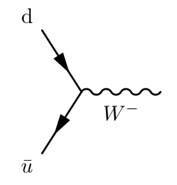
This works well for charged pion decay, for example ${\pi }^{-}\to e^{-}+{\overline{\nu }}_e$ and ${\pi }^{-}\to {\mu }^{-}+{\overline{\nu }}_{\mu }$. These imply a Feynman diagram vertex of the form shown in Fig. 11.4.

Figure 11.4: Vertex for pion decay.

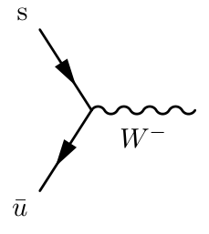
However, experimentally we also observe kaon decay, $K^{-}\to e^{-}+{\overline{\nu }}_e$ and $K^{-}\to {\mu }^{-}+{\overline{\nu }}_{\mu }$. These imply a Feynman diagram vertex of the form shown in Fig. 11.5. This means there must be quark mixing between generations. How do we account for this in our model of lepton-quark symmetry?

Figure 11.5: Vertex for kaon decay.

The resolution is that quarks can ‘mix’ (i.e. they are linear combinations of each other). The result is that the coupling strength of previously allowed vertices is modified by a factor $\cos {\theta }_c$, i.e. $g_{ud}=g_{cs}=g_W\cos {\theta }_c$, and previously forbidden vertices are now allowed with a coupling strength $g_{us}=g_{cd}=g_W\sin {\theta }_c$. The angle ${\theta }_c$ is called the Cabibbo angle and has to be measured experimentally, and ${\theta }_c=0$ would mean no quark-mixing.

One can compare the rates of hadron decays to deduce the value of the Cabibbo angle. Returning to the case of pion decay, the coupling of the $d\overline{u}W$ vertex is $g_W\cos {\theta }_c$, and for kaon decay the coupling of the $s\overline{u}W$ vertex is $g_W\sin {\theta }_c$. Since the decay rates are proportional to the square of the couplings,

$$\frac{\mathrm{\Gamma }\left(K^{-}\to e^{-}+{\overline{\nu }}_e\right)}{\mathrm{\Gamma }\left({\pi }^{-}\to e^{-}+{\overline{\nu }}_e\right)}\propto \frac{g_{us}^2}{g_{ud}^2}={\tan }^2{\theta }_c.$$ (11.12)

In reality, the decay rates are also dependent on the quark masses. A proper analysis leads to a measured Cabibbo angle of ${\theta }_c=13.1$ degrees.

11.3.2 Third generation

By adding a third generation we must allow for mixing between the quark states. The coupling between quarks can be parameterised by the following matrix

(11.13)

The couplings are given in terms of the matrix elements by $g_{\alpha \beta }=g_W{V}_{\alpha \beta }$.

The matrix (11.13) is called the Cabibbo-Kobayashi-Maskawa (CKM) matrix. For mixing between the first two generations the 2 $\times$ 2 matrix is real and specified by a single parameter (the Cabibbo angle). The more general CKM matrix is complex and is specified by four free parameters. The fact that it is complex is actually very important – this property is required for CP violation to occur in weak interactions. This in turn is crucial for our very existence. In order to generate a matter-antimatter imbalance in the early Universe CP violation must occur. Without 3 quark generations, we would have long ago annihilated, as there would be no mechanism to create more matter than anti-matter.

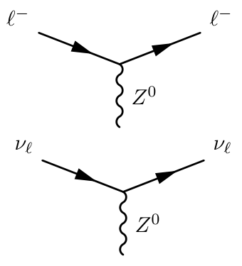
11.4 Neutral current interactions

Neutral current interactions are weak interactions involving $Z^0$ bosons. The basic vertices for $Z^0$-lepton interactions are shown in Fig. 11.6. The quark vertices can be obtained by using lepton-quark symmetry.

However, in neutral current interactions flavour changing vertices do not occur. This is also true when considering all three generations, and flavour-changing neutral currents have not been observed experimentally.

Figure 11.6: The basic vertex for $Z^0$-lepton interactions, where $\mathrm{\ell }=e,\mu ,\tau$.

11.5 Exercises

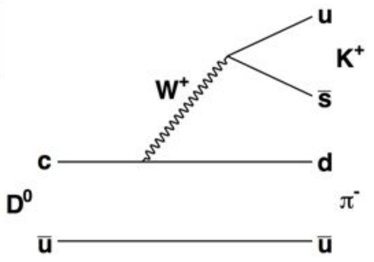
Example 11.5.1.

For the D meson decay $D^0\to K^{+}+{\pi }^{-}$, draw the lowest order Feynman diagram and indicate the coupling strength at each vertex in terms of the Cabibbo angle ${\theta }_{\mathrm{C}}$. Hence determine the decay rate in terms of ${\theta }_{\mathrm{C}}$. You can ignore the 3rd generation of quarks.

Solution.

The Feynman diagram is shown in Fig. 11.7. Note there is a $cdW$ vertex, which is Cabibbo suppressed with a coupling strength $g_W\sin {\theta }_{\mathrm{C}}$, and a $u\overline{s}W$ vertex, which is also Cabibbo suppressed with a coupling strength $g_W\sin {\theta }_{\mathrm{C}}$. The decay rate is proportional to the square of the couplings, so multiplying by each vertex and squaring, the total decay rate is $\propto g_W^4{\sin }^4{\theta }_{\mathrm{C}}$.

Figure 11.7: Feynman diagram for $D^0\to K^{+}+{\pi }^{-}$ decay.